AIR FRAME INTEGRATED SCRAMJET ENGINE INLET CONFIGURATION

1. INTRODUCTION

1.1         GENERAL

A scramjet (supersonic combustion ramjet) is a variant of a ramjet air-breathing combustion jet engine in which the combustion process takes place in supersonic airflow. As in ramjets, a scramjet relies on high vehicle speed to forcefully compress and decelerate the incoming air before combustion (hence ramjet), but whereas a ramjet decelerates the air to subsonic velocities before combustion, airflow in a scramjet is supersonic throughout the entire engine. 

This allows the scramjet to efficiently operate at hyper-sonic speeds (Mach >5) theoretical projections place the top speed of a scramjet between Mach 12 and Mach 24, which is near orbital velocity. An airframe-integrated scramjet is basically composed of three basic components: a converging air intake, where incoming air is compressed and decelerated; a combustion, where gaseous fuel is burned with atmospheric oxygen to produce heat; and a diverging nozzle, where the heated air is accelerated to produce thrust.

1.2 DEFINITION OF A SCRAMJET ENGINE

In order to provide the definition of a scramjet engine, the definition of a ramjet engine is first necessary, as a scramjet engine is a direct descendant of a ramjet engine.

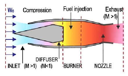
Ramjet engines have no moving parts, instead operating on compression to slow freestream supersonic air to subsonic speeds, thereby increasing temperature and pressure, and then combusting the compressed air with fuel. Lastly, a nozzle accelerates the exhaust to supersonic speeds, resulting in thrust. Figure 1 below shows a two-dimensional schematic of a ramjet engine.

Fig 1.2        TWO-DIMENSIONAL SCHEMATIC OF A RAMJET ENGINE

Due to the deceleration of the freestream air, the pressure, temperature and density of the flow entering the burner are considerably higher than in the freestream. At flight Mach numbers of around Mach 6, these increases make it inefficient to continue to slow the flow to subsonic speeds. Thus, if the flow is no longer slowed to subsonic speeds, but rather only slowed to acceptable supersonic speeds, the ramjet is then termed a supersonic combustion ramjet,‟ resulting in the acronym scramjet. Figure 2 below shows a two-dimensional schematic of a scramjet engine.

Though the concept of ramjet and scramjet engines may sound like something out of science fiction, scramjet engines have been under development for at least forty years. The following subsection will give a brief chronological history of the scramjet engine.

1.3 SCRAMJET ENGINE HISTORICAL TIMELINE

It is the intention of this section to provide a brief introduction to the historical timeline of the scramjet, so as to provide a knowledge base for the current project. There have been many authors that have provided more thorough historical accounts of both the ramjet and scramjet this section only seeks to list the highlights of the scramjet‟s development here.

As mentioned previously, the scramjet is a direct descendant of the ramjet. Therefore, in an attempt to provide a brief historical timeline of the modern-day scramjet, we must first begin with the invention of the ramjet. The first patent for a subsonic ramjet device, specifically for what is now known as an ejector ramjet, was issued to Lake in the United States in 1909 .Simultaneously, René Lorin of France was working on ejector ramjets, publishing the first treatise on subsonic ramjets in 1913 .According to Fry ,the ramjet engine reached a relative peak of interest during the 1950s in terms of the number of operational systems being deployed, with a subsequent international resurgence of attention beginning in the 1980s.

 Development on the scramjet, on the other hand, did not begin until the mid 1950s through early 1960s .The basis for its development came about due to an interest in “burning fuels in external streams to either reduce the base drag of supersonic projectiles or to produce lift and/or thrust on supersonic and hypersonic airfoils in the early 1950s. Additionally, the findings of the 1960 study by Dugger on the relative performance of a kerosene-fueled conventional ramjet engine (CRJ) and a scramjet engine showed that the scramjet‟s performance would exceed the performance of the CRJ in the speed range of Mach 6 to 8. The first scramjet demonstration also took place in 1960 byFerri . Following this demonstration, many major scramjet development programs were started in the United States, the most extensive of these being the NASA Hypersonic Research Engine or Hypersonic Ramjet Experiment (HRE) program in 1964. The core goal for the HRE project was to test a “complete, regenerative cooled, flight weight scramjet on the X-15A-2 rocket research airplane”.

Unfortunately, this program was not able to be flight tested as the cost to repair the X-15 A-2 was too high and the entire X-15 program was cancelled in 1968 . (Note: The damage referred to here occurred during the first non-burning test flight when the shock wave from the inlet spike impinged on the lower ventral fin, causing extensive damage one of the first incidents of shock-shock interaction heating, which became a major research area in itself ).However, many other projects continued towards developing the scramjet. 

In summary, the major propulsion systems of the modern era have a direct correlation between the year of their first flight and their current prevalence of application: Turbojet-1939, Ramjet-1940, High-Performance Large Liquid-Fueled Rocket Engine-1943, Practical Man-Rated Reusable Throttleable Rocket Engine-1960, and the Scramjet-2002. However, despite the fact that no operational and readily available scramjet engine currently exists, this is not due to a lack of potential applications which would benefit greatly from the use of the scramjet.

1.4  DESIGN PRINCIPLE OF A SCRAMJET ENGINE

    Scramjet engines are a type of jet engine, and rely on the combustion of fuel and an oxidizer to produce thrust. Similar to conventional jet engines, scramjet-powered aircraft carry the fuel on board, and obtain the oxidizer by the ingestion of atmospheric oxygen (as compared to rockets, which carry both fuel and an oxidizing agent). This requirement limits scramjets to suborbital atmospheric propulsion where the oxygen content of the air is sufficient to maintain combustion.

 

   The scramjet is composed of three basic components: a converging inlet, where incoming air is compressed; a combustor, where gaseous fuel is burned with atmospheric oxygen to produce heat; and a diverging nozzle, where the heated air is accelerated to produce thrust. Unlike a typical jet engine, such as a turbojet or turbofan engine, a scramjet does not use rotating, fan-like components to compress the air; rather, the achievable speed of the aircraft moving through the atmosphere causes the air to compress within the inlet. As such, no moving parts are needed in a scramjet. In comparison, typical turbojet engines require inlet fans, multiple stages of rotating compressor fans, and multiple rotating turbine stages, all of which add weight, complexity, and a greater number of failure points to the engine.
Due to the nature of their design, scramjet operation is limited to near-hypersonic velocities. As they lack mechanical compressors, scramjets require the high kinetic energy of a hypersonic flow to compress the incoming air to operational conditions. Thus, a scramjet-powered vehicle must be accelerated to the required velocity (usually about Mach 4) by some other means of propulsion, such as turbojet, railgun, or rocket engines. In the flight of the experimental scramjet-powered Boeing X-51A, the test craft was lifted to flight altitude by a Boeing B-52Stratofortress before being released and accelerated by a detachable rocket to near Mach 4.5. In May 2013, another flight achieved an increased speed of Mach 5.1

1.5 BASIC PRINCIPLE OF A SCRAMJET ENGINE

   Scramjets are designed to operate in the hypersonic flight regime, beyond the reach of turbojet engines, and, along with ramjets, fill the gap between the high efficiency of turbojets and the high speed of rocket engines. Turbo machinery based engines, while highly efficient at subsonic speeds, become increasingly inefficient at transonic speeds,as the compressor fans found in turbojet engines require subsonic speeds to operate.While the flow from transonic to low supersonic speeds can be decelerated to these conditions, doing so at supersonic speeds results in a tremendous increase in temperature and a loss in the total pressure of the flow.

 Around Mach 3–4, turbomachinery is no longer useful, and ram-style compression becomes the preferred method.Ramjets utilize high-speed characteristics of air to literally 'ram' air through an inlet diffuser into the combustor. At transonic and supersonic flight speeds, the air upstream of  the inlet is not able to move out of the way quickly enough, and is compressed within the diffuser before being diffused into the combustor. Combustion in a ramjet takes place at subsonic velocities, similar to turbojets, but the combustion products are then accelerated through a convergent-divergent nozzle to supersonic speeds. As they have no mechanical means of compression, ramjets cannot start from a standstill, and generally do not achievesufficient compression untilsupersonic flight. The lack of intricate turbomachinery allows ramjets to deal with the temperature rise associated with decelerating a supersonic flow to subsonic speeds, but this only goes so far: at near-hypersonic velocities, the temperature rise and inefficiencies discourage decelerating the flow to the magnitude found in ramjet engines
                        

Fig 1.4 SCRAMJET ENGINE OPERATION

2.  PROBLEM STATEMENT

2.1  PROBLEM DEFINITION

This chapter will provide the problem description as well as the background theory and equations necessary to address the problem at hand.

   

The above fig shows the reference geometry for our simulation analysis. The model is already predefined by the author AUGUSTO F. MOURA, MAURÍCIO A. P. ROSA Instituto de Estudos Avançados (IEAv) Departamento de Ciência e Tecnologia Aeroespacial

   A scramjet (supersonic combusting ramjet) is a variant of a ramjet air breathing jet engine in which combustion takes place in supersonic airflow. As in ramjets, a scramjet relies on high vehicle speed to forcefully compress the incoming air before combustion (hence ramjet), but a ramjet decelerates the air to subsonic velocities before combustion, while airflow in a scramjet is supersonic throughout the entire engine. This allows the scramjet to operate efficiently at extremely high speeds.

                     

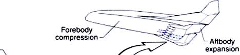
This study is concerned basically with the air intake system of an airframe-integrated scramjet engine, which is consisted of the vehicle forebody, the engine inlet and the isolator duct (see Fig.1). Although many times the isolator duct, which is located between the scramjet inlet and the combustor, is not included in analyses of the compression system, here it was considered because of the interest in knowing the airflow conditions at the combustor entrance. The isolator has the main purpose of protecting the inlet from combustor high pressure effects (adverse back pressure), although, in some situations, it also contributes to the compression process. Efficient combustion of fuel requires that supersonic airflow be supplied to the combustor at suitable pressure, temperature and flow rate. In a hypersonic vehicle with scramjet propulsion it is the air intake system that has this task.

2.2   PROPOSED SOLUTION

The work aims to present numerical simulations and performance analyses of a scramjet air intake configuration being tested for the 14-X scramjet engine when the vehicle operates at different flight speeds, altitudes and angles of attack. Besides, analyses have also been made for geometry deviations from the reference configuration, in terms of the number and angle of the intake ramps. For the numerical calculations, it has been considered 2D planar geometry and the calorically perfect gas and non-viscous models for the airflow. The goal is to have a better insight on the flow behavior in the air intake region of the propulsion system when changing flight parameters such as speed, angle of attack and altitude, for the reference configuration, and also to study the impact of intake geometry changes on the overall intake performance.

 3. LITERATURE REVIEW

3.1 DESIGN AND ANALYSIS ON SCRAMJET ENGINE                                INLETAQHEEL MURTUZA SIDDIQUI¹, G.M.SAYEED AHMED

 Research Assistant, Muffakham Jah College of Engineering & Technology., Hyderabad-500034² Senior Assistant professor, Muffakham Jah College of Engineering& Technology., Hyderabad-500034 carried out The scramjet is composed of three basic components: a converging inlet, where incoming air is compressed and decelerated; a combustor, where gaseous fuel is burned with atmospheric oxygen to produce heat; and a diverging nozzle, where the heated air is accelerated to produce thrust. Unlike a typical jet engine, such as a turbojet or turbofan engine, a scramjet does not use rotating, fan-like components to compress the air; rather, the achievable speed of the aircraft moving through the atmosphere causes the air to compress within the inlet. As such, no moving parts are needed in a scramjet. In comparison, typical turbojet engines require inlet fans, multiple stages of rotating compressor fans, and multiple rotating turbine stages, all of which add weight, complexity, and a greater number of failure points to the engine. The parts described above can be seen in Figure below.

 

Due to the nature of their design, scramjet operation is limited to near-hypersonic velocities. As they lack mechanical compressors, scramjets require the high kinetic energy of a hypersonic flow to compress the incoming air to operational conditions. Thus, a scramjet powered vehicle must be accelerated to the required velocity by some other means of propulsion, such as turbojet, railgun, or rocket engines. While scramjets are conceptually simple, actual implementation is limited by extreme technical challenges. Hypersonic flight within the atmosphere generates immense drag, and temperatures found on the aircraft and within the engine can be much greater than that of the surrounding air. Maintaining combustion in the supersonic flow presents additional challenges, as the fuel must be injected, mixed, ignited, and burned within milliseconds. While scramjet technology has been under development since the 1950s, only very recently have scramjets successfully achieved powered flight

3.2 A NUMERICAL INVESTIGATION OF  SCRAMJET

ENGINEAIR   INTAKES  FOR THE  14-X HYPERSONIC           VEHICLEAUGUSTO F. MOURA, MAURÍCIO A. P.ROSA

Instituto de EstudosAvançados(IEAv) Departamento de Ciência e Tecnologia Aeroespacial TrevoCel. Aviador José Alberto Albano do Amarante, São José dos Campos,Brasil carried outpar tofthe research and development, at the Institute for Advanced Studies (IEAv), of the first Brazilian hypersonic vehicle prototype, the 14-X airplane.It presents CFD results and performance calculations of the air intake section of some scramjet engine configurations under several operating conditions assuming 2D planar geometry. The reference case considers the vehicle flying at Mach 7 and zero angle of attack at an altitude of 30km. In thi scase, air compression is achieved by two ramps,one of which is the vehicle forebody itself and the other is a scramjet inlet compression ramp, and the engine cowl which satisfies the“shock-onlip”condition. From this reference case,several other cases were simulated varying vehicle operating conditions such as altitude, velocity and angle of attack. Besides these, calculations were made for different configurations of the scramjet inlet compression geometry by varying the inlet compression ramp angle, as well as the number of inlet compression ramps. The airflow in the intake is calculated numerically with the commercial Ansys Fluent software, considering the air as a calorically perfect gas for inviscid flow. For the intake performance analysis, several parameters characterizing the intakes have been calculated and compared.

3.3 COMPUTATIONAL ANALYSIS OF   SCRAMJET  INLET

 Murugesan, Dilip A Shah and Nirmalkumar IndiaScramjet inlets are the most vital component of the engine and their design having more effective on the overall performance of the engine. Thus, the forward capture shape of the engine inlet should conform to the vehicle body shape. A 2-D computational study for scramjet inlet with different ramp length and angles are studied to compress the air by blunted and sharp leading edge, moving the whole cowl up and down, deflecting the cowl lip and axisymmetric inlet with sharp and blunted leading edge. 

These geometric changes have produced a numerous shocks in inlet and remarkable influence on the flow in several aspects. However, the performance of these inlets tends to degrade as higher Mach number to lower Mach number. These inlets consisting of various ramps producing oblique shocks followed by a cowl shock is chosen in order to increase air mass capture and reduce spillage in scramjet inlets at Mach numbers below the design value. An impinging shock may force the boundary layer to separate from the wall, resulting in total pressure recovery losses and a reduction of the inlet efficiency. Design an inlet to meet the requirements such as Low stagnation pressure loss, High static pressure and temperature gain and deceleration of flow to a desired value of Mach number. Fixed geometry inlets can be used only over a relatively narrow range of Mach number while one method to improve this performance is to use variable-geometry inlets which can be used over a wide range of Mach number with reasonably good pressure recovery. A two dimensional analysis is carried out in this project. CATIA is used to create the model. GAMBIT is used to create the mesh. FLUENT is used to cover the flow analysis.

4. INTRODUCTION TO CFD

4.1 GENERAL

Computational Fluid Dynamics or CFD as it is popularly known, is used to generate flow simulations with the help of computers. CFD involves the solution of the governing laws of fluid dynamics numerically. The complex set of partial differential equations are solved on in geometrical domain divided into small volumes, commonly known as a mesh (or grid).CFD has enabled us to understand the world in new ways. We can now see what it is like to be in a furnace, model how blood flows through our arteries and veins and even create virtual worlds. CFD enables analysts to simulate and understand fluid flows without the help of instruments for measuring various flow variables at desired locations.

                                                       

Fluent is the CFD solver which can handle both structured grids, i.e. rectangular grids with clearly defined node indices, and unstructured grids. Unstructured grids are generally of triangular nature, but can also be rectangular. In 3-D problems, unstructured grids can consist of tetrahedral (pyramid shape), rectangular boxes, prisms, etc 

4.2 Finite - volume approach

The commercial code Fluent solve the governing integral equations for the conservation of mass and momentum, and (when appropriate) for energy and other scalars, such as turbulence and chemical species. In both cases a control-volume-based technique is used which consists of,

·        Division of the domain into discrete control volumes using a     computational grid 

·       Integration of the governing equations on the individual control volumes to construct algebraic equations for the discrete dependent variables (unknowns), such as velocities, pressure, temperature, and conserved scalars.

·      Linearization  of  the  discretion  equations  and  solution  of  the resultant linear equation system, to yield updated values of  the Fluent is a commercial 2D/3D unstructured mesh solver, which adopts Multigrid solution algorithms. It uses a co-located grid, meaning that all flow parameters are stored in the cell-centers. 

Two numerical methods are available in Fluent:

·       Pressure-based solver

·       Density-based solver 

The first one was developed for low-speed in compressible flows, whereas the second was created for the high-speed compressible flows solution. Although they have been recently modified in order to operate for a wider range of flow conditions, in the present study, which involves in compressible flows, the pressure-based approach was preferred

Pressure based solver

In the pressure-based approach the pressure field is obtained by solving a pressure correction equation, which results from combining continuity and momentum equation. i.e., the pressure equation is derived in such a way that the velocity field, corrected by the pressure, satisfies the continuity. The governing equations are non-linear and coupled one another. The solution process involves therefore iterations, wherein the entire set of governing equations is solved repeatedly, until the solution converges.

Two types of solution algorithms are available in Fluent:

·      Segregated      ·     Coupled

The segregated pressure-based solver uses a solution algorithm

Where the governing equations are solved sequentially (i.e., segregated) from one another. The segregated algorithm is memory-efficient, since the discretized equations need only be stored in the memory one at a time. However, the solution convergence is relatively slow, inasmuch as the equations are solved in a decoupled manner. Unlike the segregated algorithm described above, the pressure-based coupled algorithm solves a coupled system of equations comprising the momentum equations and the pressure-based continuity equation. The remaining equations (i.e. scalars) are solved in a decoupled fashion as in the segregated algorithm. Since the momentum and continuity equations are solved in a closely coupled manner, the rate of solution convergence significantly improves when compared to the segregated algorithm. However, the memory requirement increases by 1.5 - 2 times that of the segregated algorithm since the discrete system of all momentum and pressure-based continuity equations needs to be stored in the memory when solving for the velocity and pressure fields. For our computation, the segregated pressure-based solver has been used.

 Pressure-Velocity Coupling

      Solution of  Navier-Stokes equation is complicated even because of the lack of an independent equation for the pressure, whose gradient contribute to each of the three momentum equations. Moreover, for incompressible flows like we have been dealing with, the continuity equation does not have a dominant variable, but it is rather a kinematic constraint on the velocity field. Thus, the pressure field (the pressure Gradients when incompressible) should be generated by satisfying mass conservation. Several approaches for pressure-velocity coupling are possible. We choose the classical SIMPLE and SIMPLEC (consistent) schemes, which are useful mainly for steady computations and low-skewed grids, even if some unsteady case was run, and in spite of the high degree of distortion within the mesh. This because convergence appeared acceptable,even when compared to the PISO scheme which is usually the best option for transient computations. Proper under-relaxation factors were set for the different investigated solutions.The 

4.3 Discretization scheme

The following discretization scheme have been used within the     project

                  ·         First-Order Upwind scheme

·         Second-Order Upwind scheme

 ·         QUICK scheme

The temporal discretization used for unsteady computations was first order accurate. For pressure interpolation, the schemes adopted were the default interpolation, which computes the face pressure using momentum equation coefficients and the PRESTO (PREssure Staggering Option). The first procedure works well as long as the pressure variation between cell centres is smooth. When there are jumps or large gradients in the momentum source terms between control volumes, the pressure profile has a high gradient at the cell face, and cannot be interpolated using this scheme. Flows for which the standard pressure interpolation scheme will have trouble include flows with large body forces, such as in strongly swirling flows, natural convection and the like. In such cases, it is necessary to pack the mesh in regions of high gradient to resolve the pressure variation adequately. Another source of error is that Fluent assumes the normal pressure gradient at the wall is zero. The PRESTO scheme uses the discrete continuity balance for a staggered control volume about the face, to compute the staggered (i.e., face) pressure.

4.4 Defining Boundary Conditions

Boundary conditions (BCs) specify the flow variables on the boundaries of the chosen physical model. They are therefore a critical component of a simulation, and it is important they are specified appropriately. The utilized boundary conditions follows, named as reported in the next chapters.

            ·          Wall (no-slip)

Wall boundary condition is used to bound fluid and solid regions, for instance the blade surface in a wind turbine model. The no-slip condition is the default setting for viscous flows and the shear-stress calculation in turbulent flows follows the adopted turbulent model.

•                      Velocity-Inlet

Velocity inlet boundary conditions are used to define the flow velocity, along with all relevant scalar properties of the flow, at flow inlets. This BC is suitable for in compressible flows, whereas for compressible flows will lead to a non-physical result because stagnation conditions are floating. It is possible so set both constant and variable parameters, as well as they can be alternatively uniform or non-uniformly distributed along the boundary itself.

•                     Pressure-Outlet

It means that a specific static pressure at outlet is set, and allows also a set of backflow conditions to minimize convergence difficulties Symmetry.

It is the analogous of a zero-shear slip wall in viscous flow. Zero normal velocity is at a symmetry plane and zero normal gradients of all variables exist there as well.

4.5 Post-processing

Fluent allows a complete post-processing of solution data. Most of them are below. Moreover, the solution data can be easily exported in a number of common file formats, to be analysed with other post-processing tools.

·        Domain and grid visualization

·        Vectorial plots of solution variables

·        Linear, surface, volume integrals

·        Iso-level and contour plots of solution variables, within selected domain zones

·        Drawing two-dimensional and three-dimensional plots

·        Tracking path-lines, stream traces, etc.

Computational Fluid Dynamics (CFD) is the branch of fluid dynamics providing a cost-effective means of simulating real flows by the numerical solution of the governing equations. The governing equations for Newtonian fluid dynamics, namely the Navier-Strokes equations, have been known forever 150 years.

This chapter explains the turbulent and heat transfer numerical models used in the present study. The governing equations and boundary conditions for all studies are presented in this section. The domain is separated into small cells to form a volume mesh (or grid) using the program GAMBIT and algorithms in FLUENT are used to solve the governing equations for viscous flow, i.e. the Navier Stokes equations 

However, the development of reduced forms of these equations is still an active area of research, in practical, the turbulent closure problem of the Reynolds-averaged Navier-strokes equations. For non-Newtonian fuid dynamics, chemically reacting flows and two phase flows, the theoretical development is at less advantage stage

Experimental methods has played an important role in validating and exploring the limits of the various approximation to the governing equations, particularly wind tunnel and rig tests that provide a cost-effective alternative to full-scale testing. The flow governing equations are extremely complicated such that analytic solutions cannot be obtained for most practical applications. Computational techniques replace the governing partial differential equations with systems of algebraic equations that are much easier to solve using computers.

The steady improvement in computing power, since the 1950‟s,thus has led to the emergence of CFD. This branch of fluid dynamics complements experimental and theoretical fluid dynamics by providing cheaper means of testing fluid flow systems. It also can allow for the testing of conditions which are not possible or extremely difficult to measure experimentally and are not amenable to analytic solutions.

Applying the fundamental laws of mechanics to a fluid gives the governing equations along with the conservation of energy equation form a set of coupled, nonlinear partial differential equations. It is not possible to solve these equations analytically for most engineering problems. However, it is possible to obtain approximate computer-based solutions to the governing equations for a variety of engineering problems. This is the subject matter of Computational Fluid Dynamics
 (CFD). There are three components in CFD analysis; the pre-processor, the solver, and the post-processor. Preprocessor is defined as a program that processes input data to produce output that is used as an input to the processor. There are a number of different solution methods which are used in CFD codes. The most common, and the one on which CFD is based is known as the finite volume technique.

4.6. WHY TURBULENCE MODEL?

Fluctuations in the velocity field mix transported quantities such as momentum and energy and cause the transported quantities to fluctuate as well. These fluctuations can be of a very small scale and therefore can create extremely large computational expenses for practical engineering calculations. A modified  set of equations that require much less computational expense are used. This is done by time-averaging the instantaneous governing equations which then contain additional unknown variables. Turbulence models are needed to solve these unknown variables. These models can be classified into two types are, (i) K – ε and (ii) K – ω.

4.6.1 K-Epsilon TURBULENCE MODEL

The K-Epsilon model has become one of the most widely used turbulence models as it provides robustness, economy and reasonable accuracy for a wide range of turbulent flows. Improvements have been made to the standard model which improves its performance and two variants are available in Fluent; the RNG (renormalization group) model and the realizable model. Three versions of the K-Epsilon model will be investigated here. The standard, RNG, and realizable models have similar form with transport equations for k and ε. The two transport equations  independently solve for the turbulent velocity and length scales. The main differences between the three models are as follows;

The turbulent Prandtl Numbers governing the turbulent diffusion of k and ε.

              The generation and destruction terms in the equation for  ε.

             The method of calculating turbulent viscosity.

4.7 SOFTWARE USED

The software‟s used in this project are GAMBIT andFLUENT. GAMBITis the program used to generate the grid or mesh for the CFD solver whereas FLUENTis the CFD solver which can handle both structured grids, i.e. rectangular grids with clearly defined node indices, and unstructured grids. Unstructured grids are generally of triangular nature, but can also be rectangular. In 3-D problems, unstructured grids can consist of tetrahedral (pyramid shape), rectangular boxes, prisms, etc. Fluent is the world's largest provider of commercial computational fluid dynamics (CFD) software and services. Fluent covers general-purpose CFD software for a wide range of industrial applications, along with highly automated, specifically focused packages. FLUENT is a state-of-the-art computer program for modelling fluid flow and heat transfer in complex geometries. FLUENT provides complete mesh exibility, including the ability to solve your own problems using unstructured meshes that can be generated about complex geometries with relative ease. Supported mesh types include 2D triangular or quadrilateral, 3D tetrahedral hexahedral pyramid wedge polyhedral, and mixed (hybrid) meshes. FLUENT is ideally suited for incompressible and compressible fluid-flow simulations in complex geometries .

 4.8. BOUNDARY CONDITIONS

	Solver	Density Based – Explicit Solver
	Gradient Option	Green Gauss – Node Based
	Turbulence Model Used	K-Epsilon (Standard)
	Boundary Condition	Pressure Far-Field and Pressure outlet
	Gauge (Absolute) Pressure ;	6.386 Pa, 223 k
	Temperature
	Courant Number	0.3
	All the PDE are solved based on the	Second order Upwind scheme
	Absolute Criteria for Convergence	1x10-23
	Material	Ideal Gas

4.9 REFERENCE VALUES

The Altitude, Mach, Temperature and the corresponding Gauge Pressure have been taken from the reference journal

Table 4.2 PRESSURE, TEMPERATURE, DENSITY AND ALTITUDE VALUES

 5. RESULT AND DISCUSSION

5.1 β AND δ VARIATIONS

Ramp Angle – Considered as Beta, and Del as specified in the Picture above. We have varied number of Del angles keeping the Beta (Ramp Angle at 20 Degree constant). And Keeping the Del 10 Degree Constant Beta has been varied. 

  5.1 BASELINE HYPERSONIC INLET MODEL GENERATE GAMBIT

Table BASE LENGTH VALUE

	CASE	PARAMETER
	Length L1	657.34
	Length L2	330

Simulations have been carried out for various models by changing the inlet and ramp anglefrom the base geopmetry.

Initially anslysis have been done for the base geometry using the base reference values for Mach 1.8.

Velocity variations were also studied for the same model. It was found that the shock is excatly formed at the upper inlet engine case. Zoomed view of velocity magnitude over thebaseline model is shown in Fig 5.4 at a Mach of 1.8.

  

5.2 MODEL – 2 – HYPERSONIC INLET WITH DEL 10 DEGREE

Fig 5.5  MESHED USING TRIANGULAR AND TETRAHEDRAL ELEMENTS UNDER UNSTRUCTURED MESH SCHEME

Study is done by varying the angles. A new model is generated having the del angle as 10 keeping the ramp angle constant. Simulations have been carried out for the geometry at Mach 1.8. Resuts have been found for pressure and velocity distribution for the model. The below figures shows the variation of pressure and  velocity distribution.

Fig 5.5 shows the generation of mes created for the model. Triangular and Tetrahedral mesh was created over the geometry to capture the model for the simulation.

Analysis  have  been  carried  out  for  the  gometry  with  del  angle  10.

Simulation results are shown in the below Figures.

Zoomed simulated view of static pressure over the model with del 10 degree when experiencing Mach 1.8 is shown in Fig 5.6. it is clearly seen that the shock is formed at both the angles and pressure difference can be studied from the contour.

Zoomed view of velocity magnitude over the model with del 10 deg when experiencing  mach 1.8 is shown in Fig 5.7 

5.3 HYPERSONIC INLET MODEL CONFIGURATION WITH DEL     5  DEGREE GENERATED IN GAMBIT

A new case model is studied for various Mach numbers by changing the del angle as 5 degree. The geometry created is shown in the Fig 5.8.

Pressure and velocity variations have been studied for the model.

The Mach number is kept constantn for this case study.       

By keeping the Mach 1.8 pressure and velocity distribution inside the inlet have been studied by comparing with the previous case. It can clealy seen from the simulations results that the compression ration have been increased inside the inlet geometry. This difference is created due to the varaition in the del angle made in the geomtery.

Zoomed view of pressure over the hypersonic inlet model configuration with del 5 degree when experiencing Mach 1.8. Zoomed view of velocity magnitude over the hypersonic inlet model configuration with del 5 degree when experiencing Mach 1.8 is shown in Figure 5.10.

5.4 HYPERSONIC INLET MODEL CONFIG WITH DEL 15 DEGREE GENERATED IN GAMBIT

Here the del angle is varied to 15 degree. The variation in the geomtery is shown in the Fig 5.11.

Simulations have been carried out for the model having del angle as 15 degree at Mach 1.8. the pressure distribution and velocity variations have been studied.

Zoomed view of static pressure over the hypersonic inlet model configuration with del 15 degree when experiencing Mach 1.8 is shown in Figure 5.12

Simulations have been carried out for the model having del angle as 20 degree at Mach 1.8. the pressure distribution and velocity variations have been studied.

Zoomed view of velocity magnitude over the hypersonic inlet model configuration with del 15 degree when experiencing Mach 1.8 is shown in Fig 5.13

1. 5.5 HYPERSONIC INLET MODEL CONFIGURATION WITH DEL 20 DEGREE GENERATED IN GAMBIT

Here the del angle is varied to 20 degree. The variation in the geomtery is shown in the Fig 5.14

Zoomed view of static pressure over the hypersonic inlet model configuration with del 20 degree when experiencing Mach 1.8 is shown in Fig 5.15

The del angle is varied from 5 degree to 20 degree and analysis have been carried out. For all the cases pressure distribution and velocity variations were studeid.

From the study it is clearly seen that for del angle of 10 degree we have got a good compression ratio. This can be clearly seen from the various pressure and velocity contours shown in the above figures for all cases.

5.6  HYPERSONIC INLET   CONFIGURATION  WITH  DEL  10 DEGREE AND BETA (RAMP ANGLE) 25 DEG GENERATED IN GAMBIT

The next set of study is done by keeping the del angle constant and varying the ramp angle from 25 degrees to 35 degrees with a variation of 5 degree at each case.

The Fig 5.17 shows the basic variation of ramp angle which is started at 25 degree having the other dimensions constant.

Zoomed view of static pressure over the hypersonic inlet configuration with del 10 degree and beta (ramp angle) 25 deg when experiencing Mach 1.8 is shown in Fig 5.18.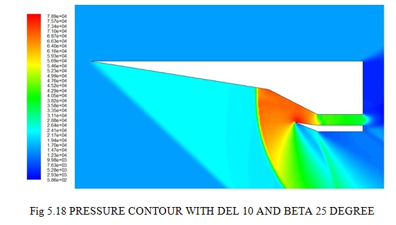

Zoomed view of velocity contours over the hypersonic inlet configuration with del 10 degree and beta (ramp angle) 25 deg when experiencing Mach 1.8 is shown in Fig 5.19.

5.7 HYPERSONIC  INLET  CONFIGURATION  WITH  DEL  10 DEGREE AND BETA (RAMP ANGLE) 30 DEG   GENERATED IN GAMBIT

The next set of sytudy is done by keeping the del angle constant and varing the ramp angle from 25 degrees to 35 degrees with a variation of 5 degree at each case. The Fig 5.17 shows the basic variation of ramp angle which is started at 30 degree having the other dimensions constant.

Zoomed view of static pressure over the hypersonic inlet configuration with del 10 degree and beta (ramp angle) 30 deg when experiencing Mach 1.8 is shown in Fig 5.21. Zoomed view of velocity contours over the hypersonic inlet configuration with del 10 degree and beta (ramp angle) 30 deg when experiencing Mach 1.8 is shown in Fig 5.22

5.8  HYPERSONIC  INLET  CONFIGURATION  WITH  DEL  10 DEGREE AND BETA (RAMP ANGLE) 35 DEG GENERATED IN GAMBIT

The next set of sytudy is done by keeping the del angle constant and varing the ramp angle from 25 degrees to 35 degrees with a variation of 5 degree at each case.

The Fig 5.17 shows the basic variation of ramp angle which is started at 35 degree having the other dimensions constant. 

Zoomed view of pressure contours over the hypersonic inlet configuration with del 10 degree and beta (ramp angle) 35 deg when experiencing Mach 1.8 is shown in Fig 5.24

Zoomed view of velocity contour over the hypersonic inlet configuration with del 10 degree and beta (ramp angle)35 deg when experiencing Mach 1.8 is shown in Fig 5.25

From all the above study it been found that having the beta angle of 25 degree gives a better compression ratio with less separation.

The values obtained from the simulation results are tabulated in the Table 5.1 and 5.2.

Hence, while varying (delta) the inlet angle, it has been observed that (increased in the delta) angle creates a formation of local shock and thereby causes compression. Whereas, at the same time greater the increase in delta angle the reflection and the interaction of the shocks degrades/distorts the uniformity of the flow and thereby reduces compression which is evident from the above table.

Increase in delta angle =decrease in static pressure

Therefore based on the required design velocity at the chamber, the optimum one can be selected. Here, delta 10 degree can be selected because it achieves maximum compression and maximum velocity. So delta 10 degree is suitable for supersonic flows.

The above table 5.2 shows the optimum pressure and velocity values from the pressure and contour plots

6. CONCLUSION

The purpose of this paper was to determine at which angle scramjet engine will achieves the maximum compression and maximum velocity by eliminating the combustion instability of the propulsion system while performance is maintained in the same flow path at the higher. And to define how, it could be accomplished. Hence a scramjet engine was then modelled in GAMBIT and analysis was carried out in FLUENT for the same with different models.

It was found that the delta angle 10 degree was feasible as it matched the theoretical values with CFD values. By this analysis we can conclude k-epsilon turbulence model exactly simulates the flow field characteristics in Supersonic and hypersonic condition in capturing shocks at leading edges and shock trains in the isolator and etc.

   In future scope in the design of this particular scramjet engine, we can varying the Mach number and varying ramp to determine the appropriate inlet performance. Preliminary results revealed that ramp angle of 25 degree shows good performance relative to the other configurations.

REFERENCES

FUTURE SCOPE

 Ø 1 .     Heiser, William H., David T. Pratt, Daniel H. Daley, and                     Unmeel B. Mehta. Hypersonic Airbreathing Propulsion.                         Washington, D.C.: American Institute of Aeronautics and                       Astronautics, 1994.

  

Ø Curran, Edward T.Scramjet Engines: The First Forty Years. Journal of Propulsion and Power, Volume 17, No. 6, November-December 2001.

Ø Fry, Ronald S.A Century of Ramjet Propulsion Technology Evolution. Journal of Propulsion and Power, Volume 20, No. 1, January-February 2004: 27-58.

Ø Waltrup, Paul J. Upper Bounds on the Flight Speed of Hydrocarbon-Fuelled Scramjet-Powered Vehicles. Journal of Propulsion and Power, Volume 17, No. 6, November-December 2001: 1199-1204.

Ø Builder, C.H. On the Thermodynamic Spectrum of Airbreathing

Ø Propulsion AIAA 1st Annual Meeting, Washington, D.C., June 1964.AIAA Paper 64-243.

Ø Heiser, William H., David T. Pratt, Daniel H. Daley, and Unmeel B. Mehta. Brief Description of the HAP Software Package. ReadMe File for Hypersonic Airbreathing Propulsion Software Package. Washington, D.C.: American Institute of Aeronautics and Astronautics, 1994

Ø     Zucrow, Maurice J., and Joe D. Hoffman. Gas Dynamics. Vol. 1. New York: John Wiley & Sons, Inc., 1976.

Ø       Anderson, Jr., John D. Modern Compressible Flow with Historical erspective. 2nd Ed. New York: McGraw-Hill

     Company, 1990 

Ø Analysis And Design Of A Hypersonic Scramjet Engine With A Starting Mach Number Of 4.00 By Kristen Nicole Roberts. August 2008